

Feasibility of Arbitrary Return


As a Data Scientist, when I started working on quantitative trading at Eveince, my biggest problem was quantifying the problem’s objective function. One way is to set a KPI and evaluate the performance accordingly. However, KPI definition is the challenging part in addition to finding a model that satisfies it.
The beauty of this problem is that all traders, hedge funds, and entities that want to trade on the financial markets want to increase their returns as much as possible. Once they use return as their evaluation metric, they get caught in a dangerous trap! Imagine that you know you want something and do your best to reach it, but you can not measure your distance from it. How can you measure your progress?
After studying the evaluation of systematic trading entities, you may understand that this problem is a different animal! We cannot evaluate our system using traditional problem metrics, or they are not enough. There are numerous and variant evaluation metrics to assess the performance of a trader; in other words, which portfolio is more trustable/attractive to invest in it. Sharper Ratio, Sortino Ratio, Alpha Ratio, Beta Ratio, Maximum Drawdown, Probability of N% loss, success Rate, etc.. are some examples of evaluation metrics as mentioned earlier.
Despite all of these powerful and sometimes complicated metrics, there is still one important question. Can a trader (any type of them, quantitative trader, hedge fund, fundamental trader, etc.) guarantee a specific return to its customer? Not only to customers for marketing purposes, but also to their department or team? Is it possible to set a ‘return’ goal in the financial market and plan to reach it? For example, is it possible to say, ‘we want to gain a 300% Return in the FX market next year? Or can our team guarantee a 500 % annualized return in the cryptocurrency market? Usually, these questions are essential to those who want to collect AUM and implement their proposed trading strategy. In other words, the main question is, “is it feasible to gain an arbitrary target return during a specific period in a particular market?”
To answer this question, we should first agree that the environment of the problem is a probabilistic one. We should evaluate entities’ strategies instead of their decisions in probabilistic environments. P.s: I use strategy as a set of decisions during a specific period. Let’s consider one example:
Consider a coin toss game; if you win, you will receive +X$, and if you lose, you should pay -X$. If the coin is fair ( the probability of head and tail is the same and equal to 0.5), your expected value is 0. Theoretically, if you play N times and N is large enough, your balance will not change. Also, if you play with an unfair coin and the probability of your win is more than 0.5, your portfolio will be positive if you play enough sets. We can make the game more complicated and dynamically change the probability of appearing head and tail. Also, change the rewards per set. Therefore, Depending on how you play each hand (i.e., if you only play positive expected value), we can ‘Theoretically’ measure your gain after enough played sets. The decisions you make in this game and their rationality define your strategy.
The purpose of the mentioned example was to emphasize that we measure strategies’ theoretical expected gain in the probabilistic environments.
Therefore to model the main question, we can relax the financial market’s problem as a coin toss game. Instead of flipping a coin, you decide to create a position or not(here, we assume that our decisions are independent as flipping the coin is). The expectation of winning is a function of two following parameters:
your algorithms/mechanism success rate ( which can be calculated by past decisions)
market reward behavior (which can be modeled as return distribution of market and commission rate).
To check the feasibility of target return during a specific period (i.e., next year), In addition to the above issues, the number of decisions ( number of games played, number of positions, number of bets) matters which can be represented as period Time.
We can assume an equation that can check the feasibility of target return in a specific period by considering mentioned parameters, Figure 1.

Let’s review this modeling with an experimental setup. Suppose we have built an Algo-trading bot that trades Bitcoin by considering the following assumptions:
We have a model that trades on the bitcoin market and decides to buy or sell an asset.
The model’s order will be executed each day.
Bet sizing strategy (bet sizing means the approach that we determine an order’s size when we want to place a buy/sell order) is to put all assets on either the buy or sell side.
We manage assets in a compound approach (It means all gains or losses that are obtained by each decision would be participating in the next decision)
Due to the compound strategy, the strategy’s total return follows the below equation.

Where Ri is the return of each trade and decision, T is the count of our all decision during the target period. Note that we are going to decide on each timestamp (i.e., Each day). Decisions like buying an asset, selling it, or even holding and doing nothing affect the total portfolio that a return can represent. In addition, because we assumed our bet sizing is using the entire of our asset during each bet, therefore:

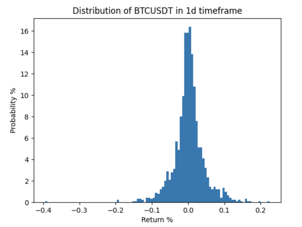
Which is calculated with a 1day sampling resolution and is illustrated in Figure 2.
Note that our model enables us to sample returns from distribution, not uniformly. So we can rewrite equation 1 into :

It is clear that N+P = T (all of our decisions lead to positive or negative returns and nothing else). On the other hand, we can estimate the model’s success rate by its performance in the past. So we could determine P/T and N/T=1-P/T ratios.
By considering measurable factors: Success Rate (P/T), Market Return Distributions, Target Period (T) we can easily simulate multiple scenarios and speculate return expectations during the target period. considering a flip coin game, on each hand, you have P/T chance to win, and if you win, you can pick up Ri randomly from the market return distribution, and in case of losing, vice versa. We can run this scenario K times and generate several scenarios, Figure3.

We can also calculate the final return distribution by obtaining the K scenarios’ final result, Figure 4. the distribution can give us information about the confidence and feasibility of targeting a specific return. Also, we can change the parameters ( success rate, T, market. distribution) to see what happens for distribution and the feasibility of target return. Like all probabilistic problems, the feasibility of a phenomena’s occurrence should be evaluated by statistical measures, like expectations and variance, kurtosis, skewness, etc., which helps us quantify distributions.

The above simulation explained modeling to check the feasibility of arbitrary return by existing model and strategy. We can use this methodology to answer different questions or compare different types of strategies.
For example, we can compare a compound strategy vs a non-compound one and answer the following questions: why compound strategy? Is it always preferable to use a compound strategy? Based on our model predictive power, periods to trade, or market behavior ( market return distribution), can we use a non-compound strategy instead?
Consider that the mentioned example was configured for compound strategy.
so we can write the expected return of the above setup as :

Respectfully, we can quickly write equation 4 for non-compound strategy as below:

Therefore:

By setting the parameters in the above inequality and checking the expected returns (other statistical measures, like std and skewness can also be considered to achieve trustable comparison) we can decide to use a compound or a non-compound strategy based on the market during a target period by our existing estimator model.
It is important to note that we assume that our decisions are independent as flipping the coin is, which may not be a valid hypothesis based on the strategy’s characteristics. There is another assumption that the model estimator is independent of market returns. In other words, some models or methods consider market volatility, which leads them to predict more significant returns more accurately than small ones, or vice versa. It is better to consider the relation between returns gained by models and market return distributions to address this issue. Quant researchers can use tools like alpha and beta or some sort of them to evaluate the systematic risk (relation) between the two mentioned variables to address this issue.
 | A guest post by
|